A history of the calculus
The main ideas which underpin the calculus developed over a very long period of time indeed. The first steps were taken by Greek mathematicians.
To the Greeks numbers were ratios of integers so the number line had "holes" in it. They got round this difficulty by using lengths, areas and volumes in addition to numbers for, to the Greeks, not all lengths were numbers.
Zeno of Elea, about 450 BC, gave a number of problems which were based on the infinite. For example he argued that motion is impossible:-
However Archimedes, around 225 BC, made one of the most significant of the Greek contributions. His first important advance was to show that the area of a segment of a parabola is the area of a triangle with the same base and vertex and of the area of the circumscribed parallelogram. Archimedes constructed an infinite sequence of triangles starting with one of area and continually adding further triangles between the existing ones and the parabola to get areas
The area of the segment of the parabola is therefore
Archimedes used the method of exhaustion to find an approximation to the area of a circle. This, of course, is an early example of integration which led to approximate values of π.
Among other 'integrations' by Archimedes were the volume and surface area of a sphere, the volume and area of a cone, the surface area of an ellipse, the volume of any segment of a paraboloid of revolution and a segment of an hyperboloid of revolution.
No further progress was made until the 16th Century when mechanics began to drive mathematicians to examine problems such as centres of gravity. Luca Valerio (1552-1618) published De quadratura parabolae Ⓣ in Rome (1606) which continued the Greek methods of attacking these type of area problems. Kepler, in his work on planetary motion, had to find the area of sectors of an ellipse. His method consisted of thinking of areas as sums of lines, another crude form of integration, but Kepler had little time for Greek rigour and was rather lucky to obtain the correct answer after making two cancelling errors in this work.
Three mathematicians, born within three years of each other, were the next to make major contributions. They were Fermat, Roberval and Cavalieri. Cavalieri was led to his 'method of indivisibles' by Kepler's attempts at integration. He was not rigorous in his approach and it is hard to see clearly how he thought about his method. It appears that Cavalieri thought of an area as being made up of components which were lines and then summed his infinite number of 'indivisibles'. He showed, using these methods, that the integral of from 0 to was by showing the result for a number of values of and inferring the general result.
Roberval considered problems of the same type but was much more rigorous than Cavalieri. Roberval looked at the area between a curve and a line as being made up of an infinite number of infinitely narrow rectangular strips. He applied this to the integral of from 0 to 1 which he showed had approximate value
Fermat was also more rigorous in his approach but gave no proofs. He generalised the parabola and hyperbola:-
Fermat also investigated maxima and minima by considering when the tangent to the curve was parallel to the -axis. He wrote to Descartes giving the method essentially as used today, namely finding maxima and minima by calculating when the derivative of the function was 0. In fact, because of this work, Lagrange stated clearly that he considers Fermat to be the inventor of the calculus.
Descartes produced an important method of determining normals in La Géométrie Ⓣ in 1637 based on double intersection. De Beaune extended his methods and applied it to tangents where double intersection translates into double roots. Hudde discovered a simpler method, known as Hudde's Rule, which basically involves the derivative. Descartes' method and Hudde's Rule were important in influencing Newton.
Huygens was critical of Cavalieri's proofs saying that what one needs is a proof which at least convinces one that a rigorous proof could be constructed. Huygens was a major influence on Leibniz and so played a considerable part in producing a more satisfactory approach to the calculus.
The next major step was provided by Torricelli and Barrow. Barrow gave a method of tangents to a curve where the tangent is given as the limit of a chord as the points approach each other known as Barrow's differential triangle.
Both Torricelli and Barrow considered the problem of motion with variable speed. The derivative of the distance is velocity and the inverse operation takes one from the velocity to the distance. Hence an awareness of the inverse of differentiation began to evolve naturally and the idea that integral and derivative were inverses to each other were familiar to Barrow. In fact, although Barrow never explicitly stated the fundamental theorem of the calculus, he was working towards the result and Newton was to continue with this direction and state the Fundamental Theorem of the Calculus explicitly.
Torricelli's work was continued in Italy by Mengoli and Angeli.
Newton wrote a tract on fluxions in October 1666. This was a work which was not published at the time but seen by many mathematicians and had a major influence on the direction the calculus was to take. Newton thought of a particle tracing out a curve with two moving lines which were the coordinates. The horizontal velocity and the vertical velocity were the fluxions of and associated with the flux of time. The fluents or flowing quantities were and themselves. With this fluxion notation was the tangent to .
In his 1666 tract Newton discusses the converse problem, given the relationship between and find . Hence the slope of the tangent was given for each and when then Newton solves the problem by antidifferentiation. He also calculated areas by antidifferentiation and this work contains the first clear statement of the Fundamental Theorem of the Calculus.
Newton had problems publishing his mathematical work. Barrow was in some way to blame for this since the publisher of Barrow's work had gone bankrupt and publishers were, after this, wary of publishing mathematical works! Newton's work on Analysis with infinite series was written in 1669 and circulated in manuscript. It was not published until 1711. Similarly his Method of fluxions and infinite series was written in 1671 and published in English translation in 1736. The Latin original was not published until much later.
In these two works Newton calculated the series expansion for and and the expansion for what was actually the exponential function, although this function was not established until Euler introduced the present notation .
You can see graphs of the series expansions for sine at THIS LINK and for cosine at THIS LINK. They are now called Taylor or Maclaurin series.
Newton's next mathematical work was Tractatus de Quadratura Curvarum Ⓣ which he wrote in 1693 but it was not published until 1704 when he published it as an Appendix to his Optiks. This work contains another approach which involves taking limits. Newton says
Leibniz learnt much on a European tour which led him to meet Huygens in Paris in 1672. He also met Hooke and Boyle in London in 1673 where he bought several mathematics books, including Barrow's works. Leibniz was to have a lengthy correspondence with Barrow. On returning to Paris Leibniz did some very fine work on the calculus, thinking of the foundations very differently from Newton.
Newton considered variables changing with time. Leibniz thought of variables as ranging over sequences of infinitely close values. He introduced and as differences between successive values of these sequences. Leibniz knew that gives the tangent but he did not use it as a defining property.
For Newton integration consisted of finding fluents for a given fluxion so the fact that integration and differentiation were inverses was implied. Leibniz used integration as a sum, in a rather similar way to Cavalieri. He was also happy to use 'infinitesimals' and where Newton used and which were finite velocities. Of course neither Leibniz nor Newton thought in terms of functions, however, but both always thought in terms of graphs. For Newton the calculus was geometrical while Leibniz took it towards analysis.
Leibniz was very conscious that finding a good notation was of fundamental importance and thought a lot about it. Newton, on the other hand, wrote more for himself and, as a consequence, tended to use whatever notation he thought of on the day. Leibniz's notation of and ∫ highlighted the operator aspect which proved important in later developments. By 1675 Leibniz had settled on the notation
After Newton and Leibniz the development of the calculus was continued by Jacob Bernoulli and Johann Bernoulli. However when Berkeley published his Analyst in 1734 attacking the lack of rigour in the calculus and disputing the logic on which it was based much effort was made to tighten the reasoning. Maclaurin attempted to put the calculus on a rigorous geometrical basis but the really satisfactory basis for the calculus had to wait for the work of Cauchy in the 19th Century.
To the Greeks numbers were ratios of integers so the number line had "holes" in it. They got round this difficulty by using lengths, areas and volumes in addition to numbers for, to the Greeks, not all lengths were numbers.
Zeno of Elea, about 450 BC, gave a number of problems which were based on the infinite. For example he argued that motion is impossible:-
If a body moves from A to B then before it reaches B it passes through the mid-point, say of AB. Now to move to it must first reach the mid-point of . Continue this argument to see that A must move through an infinite number of distances and so cannot move.Leucippus, Democritus and Antiphon all made contributions to the Greek method of exhaustion which was put on a scientific basis by Eudoxus about 370 BC. The method of exhaustion is so called because one thinks of the areas measured expanding so that they account for more and more of the required area.
However Archimedes, around 225 BC, made one of the most significant of the Greek contributions. His first important advance was to show that the area of a segment of a parabola is the area of a triangle with the same base and vertex and of the area of the circumscribed parallelogram. Archimedes constructed an infinite sequence of triangles starting with one of area and continually adding further triangles between the existing ones and the parabola to get areas
The area of the segment of the parabola is therefore
.
This is the first known example of the summation of an infinite series.
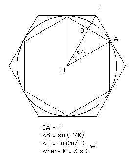
Archimedes used the method of exhaustion to find an approximation to the area of a circle. This, of course, is an early example of integration which led to approximate values of π.
Here is Archimedes' diagram for approximating the area of a circle
Among other 'integrations' by Archimedes were the volume and surface area of a sphere, the volume and area of a cone, the surface area of an ellipse, the volume of any segment of a paraboloid of revolution and a segment of an hyperboloid of revolution.
No further progress was made until the 16th Century when mechanics began to drive mathematicians to examine problems such as centres of gravity. Luca Valerio (1552-1618) published De quadratura parabolae Ⓣ in Rome (1606) which continued the Greek methods of attacking these type of area problems. Kepler, in his work on planetary motion, had to find the area of sectors of an ellipse. His method consisted of thinking of areas as sums of lines, another crude form of integration, but Kepler had little time for Greek rigour and was rather lucky to obtain the correct answer after making two cancelling errors in this work.
Three mathematicians, born within three years of each other, were the next to make major contributions. They were Fermat, Roberval and Cavalieri. Cavalieri was led to his 'method of indivisibles' by Kepler's attempts at integration. He was not rigorous in his approach and it is hard to see clearly how he thought about his method. It appears that Cavalieri thought of an area as being made up of components which were lines and then summed his infinite number of 'indivisibles'. He showed, using these methods, that the integral of from 0 to was by showing the result for a number of values of and inferring the general result.
Roberval considered problems of the same type but was much more rigorous than Cavalieri. Roberval looked at the area between a curve and a line as being made up of an infinite number of infinitely narrow rectangular strips. He applied this to the integral of from 0 to 1 which he showed had approximate value
.
Roberval then asserted that this tended to as tends to infinity, so calculating the area.
Fermat was also more rigorous in his approach but gave no proofs. He generalised the parabola and hyperbola:-
Parabola: to
Hyperbola: to .
In the course of examining , Fermat computed the sum of from to .
Hyperbola: to .
Fermat also investigated maxima and minima by considering when the tangent to the curve was parallel to the -axis. He wrote to Descartes giving the method essentially as used today, namely finding maxima and minima by calculating when the derivative of the function was 0. In fact, because of this work, Lagrange stated clearly that he considers Fermat to be the inventor of the calculus.
Descartes produced an important method of determining normals in La Géométrie Ⓣ in 1637 based on double intersection. De Beaune extended his methods and applied it to tangents where double intersection translates into double roots. Hudde discovered a simpler method, known as Hudde's Rule, which basically involves the derivative. Descartes' method and Hudde's Rule were important in influencing Newton.
Huygens was critical of Cavalieri's proofs saying that what one needs is a proof which at least convinces one that a rigorous proof could be constructed. Huygens was a major influence on Leibniz and so played a considerable part in producing a more satisfactory approach to the calculus.
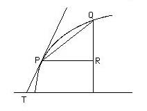
The next major step was provided by Torricelli and Barrow. Barrow gave a method of tangents to a curve where the tangent is given as the limit of a chord as the points approach each other known as Barrow's differential triangle.
Here is Barrow's differential triangle
Both Torricelli and Barrow considered the problem of motion with variable speed. The derivative of the distance is velocity and the inverse operation takes one from the velocity to the distance. Hence an awareness of the inverse of differentiation began to evolve naturally and the idea that integral and derivative were inverses to each other were familiar to Barrow. In fact, although Barrow never explicitly stated the fundamental theorem of the calculus, he was working towards the result and Newton was to continue with this direction and state the Fundamental Theorem of the Calculus explicitly.
Torricelli's work was continued in Italy by Mengoli and Angeli.
Newton wrote a tract on fluxions in October 1666. This was a work which was not published at the time but seen by many mathematicians and had a major influence on the direction the calculus was to take. Newton thought of a particle tracing out a curve with two moving lines which were the coordinates. The horizontal velocity and the vertical velocity were the fluxions of and associated with the flux of time. The fluents or flowing quantities were and themselves. With this fluxion notation was the tangent to .
In his 1666 tract Newton discusses the converse problem, given the relationship between and find . Hence the slope of the tangent was given for each and when then Newton solves the problem by antidifferentiation. He also calculated areas by antidifferentiation and this work contains the first clear statement of the Fundamental Theorem of the Calculus.
Newton had problems publishing his mathematical work. Barrow was in some way to blame for this since the publisher of Barrow's work had gone bankrupt and publishers were, after this, wary of publishing mathematical works! Newton's work on Analysis with infinite series was written in 1669 and circulated in manuscript. It was not published until 1711. Similarly his Method of fluxions and infinite series was written in 1671 and published in English translation in 1736. The Latin original was not published until much later.
In these two works Newton calculated the series expansion for and and the expansion for what was actually the exponential function, although this function was not established until Euler introduced the present notation .
You can see graphs of the series expansions for sine at THIS LINK and for cosine at THIS LINK. They are now called Taylor or Maclaurin series.
Newton's next mathematical work was Tractatus de Quadratura Curvarum Ⓣ which he wrote in 1693 but it was not published until 1704 when he published it as an Appendix to his Optiks. This work contains another approach which involves taking limits. Newton says
In the time in which x by flowing becomes , the quantity becomes i.e. by the method of infinite series,At the end he lets the increment vanish by 'taking limits'.
Leibniz learnt much on a European tour which led him to meet Huygens in Paris in 1672. He also met Hooke and Boyle in London in 1673 where he bought several mathematics books, including Barrow's works. Leibniz was to have a lengthy correspondence with Barrow. On returning to Paris Leibniz did some very fine work on the calculus, thinking of the foundations very differently from Newton.
Newton considered variables changing with time. Leibniz thought of variables as ranging over sequences of infinitely close values. He introduced and as differences between successive values of these sequences. Leibniz knew that gives the tangent but he did not use it as a defining property.
For Newton integration consisted of finding fluents for a given fluxion so the fact that integration and differentiation were inverses was implied. Leibniz used integration as a sum, in a rather similar way to Cavalieri. He was also happy to use 'infinitesimals' and where Newton used and which were finite velocities. Of course neither Leibniz nor Newton thought in terms of functions, however, but both always thought in terms of graphs. For Newton the calculus was geometrical while Leibniz took it towards analysis.
Leibniz was very conscious that finding a good notation was of fundamental importance and thought a lot about it. Newton, on the other hand, wrote more for himself and, as a consequence, tended to use whatever notation he thought of on the day. Leibniz's notation of and ∫ highlighted the operator aspect which proved important in later developments. By 1675 Leibniz had settled on the notation
written exactly as it would be today. His results on the integral calculus were published in 1684 and 1686 under the name 'calculus summatorius', the name integral calculus was suggested by Jacob Bernoulli in 1690.
After Newton and Leibniz the development of the calculus was continued by Jacob Bernoulli and Johann Bernoulli. However when Berkeley published his Analyst in 1734 attacking the lack of rigour in the calculus and disputing the logic on which it was based much effort was made to tighten the reasoning. Maclaurin attempted to put the calculus on a rigorous geometrical basis but the really satisfactory basis for the calculus had to wait for the work of Cauchy in the 19th Century.
References (show)
- K Andersen, Precalculus, 1635-1665, in I Grattan-Guinness (ed.), Companion Encyclopedia of the History and Philosophy of the Mathematical Sciences (London, 1994), 292-307.
- R T W Arthur, Newton's fluxions and equably flowing time, Stud. Hist. Philos. Sci. 26 (2) (1995), 323-351.
- M E Baron, The origins of the infinitesimal calculus (New York, 1987).
- M Blay, Deux moments de la critique du calcul infinitésimal : Michel Rolle et George Berkeley : Etudes sur l'histoire du calcul infinitésimal, Rev. Histoire Sci. 39 (3) (1986), 223-253.
- C B Boyer, The History of the Calculus and Its Conceptual Development (New York, 1959).
- W Breidert, Berkeleys Kritik an der Infinitesimalrechnung, in 300 Jahre 'Nova methodus' von G W Leibniz (1684-1984) (Wiesbaden, 1986), 185-191.
- C H Edwards, The Historical Development of the Calculus (New York, 1979).
- J O Fleckenstein, The line of descent of the infinitesimal calculus in the history of ideas, Arch. Internat. Hist. Sci. (N.S.) 3 (1950), 542-554.
- E Giusti, A comparison of infinitesimal calculus in Leibniz and Newton (Italian), Rend. Sem. Mat. Univ. Politec. Torino 46 (1) (1988), 1-29.
- N Guicciardini, Three traditions in the calculus : Newton, Leibniz and Lagrange, in I Grattan-Guinness (ed.), Companion Encyclopedia of the History and Philosophy of the Mathematical Sciences (London, 1994), 308-317.
- N Guicciardini, The Development of Newtonian Calculus in Britain, 1700-1800 (Cambridge, 1989).
- T Guitard, On an episode in the history of the integral calculus, Historia Mathematica 14 (2) (1987), 215-219.
- P Kitcher, Fluxions, limits, and infinite littlenesse : A study of Newton's presentation of the calculus, Isis 64 (221) (1973), 33-49.
- S Krämer, Zur Begründung des Infinitesimalkalküls durch Leibniz, Philos. Natur. 28 (2) (1991), 117-146.
- A Pérez de Laborda, Newtons Fluxionsrechnung im Vergleich zu Leibniz' Infinitesimalkalkül, in 300 Jahre 'Nova methodus' von G W Leibniz (1684-1984) (Wiesbaden, 1986), 239-257.
- J A van Maanen, Die Mathematik in den Niederlanden im 17. Jahrhundert und ihre Rolle in der Entwicklungsgeschichte der Infinitesimalrechnung, in 300 Jahre 'Nova methodus' von G W Leibniz (1684-1984) (Wiesbaden, 1986), 1-13.
- A Nikolic, Space and time in the apparatus of infinitesimal calculus, Zb. Rad. Prirod.-Mat. Fak. Ser. Mat. 23 (1) (1993), 199-218.
- L Pepe, Les mathématiciens italiens et le calcul infinitésimal au début du XVIIIe siècle, in 300 Jahre 'Nova methodus' von G W Leibniz (1684-1984) (Wiesbaden, 1986), 192-201.
- L Pepe, The infinitesimal calculus in Italy at the beginning of the 18th century (Italian), Boll. Storia Sci. Mat. 1 (2) (1981), 43-101.
- J Pieters, Origines de la découverte par Leibniz du calcul infinitésimal, in Cahiers du Centre de Logique 2 (Louvain-la-Neuve, 1981), 1-22.
- A Rosenthal, The history of calculus, The American Mathematical Monthly 58 (1951), 75-86.
- C J Scriba, The inverse method of tangents. A dialogue between Leibniz and Newton (1675-1677), Archive for History of Exact Sciences 2 (1964), 113-137.
- A B Shtykan, On the question of the origin of the differential and integral calculus (Russian), Voprosy Istor. Estestvoznan. i Tekhn. (3) (1986), 87-93.
- G C Smith, Thomas Bayes and fluxions, Historia Mathematica 7 (4) (1980), 379-388.
- R Thiele, Carnots Betrachtungen über die Grundlagen der Infinitesimalrechnung, in Rechnen mit dem Unendlichen (Basel, 1990), 79-94.
- O Toeplitz, The Calculus: A Genetic Approach (1963).
- J Vernet, The infinitesimal calculus and Spanish mathematics of the 18th century (Spanish), Arch. Internat. Histoire Sci. 25 (97) (1975), 304-308.
- D T Whiteside, Patterns of mathematical thought in the later seventeenth century, Archive for History of Exact Sciences 1 (1960), 179-388.
Additional Resources (show)
Other pages about Calculus history:
Other websites about Calculus history:
Written by J J O'Connor and E F Robertson
Last Update February 1996
Last Update February 1996